The pyveg Package
Introduction
The pyveg package is developed to study the evolution of vegetation patterns in semi-arid environments using data downloaded from Google Earth Engine.
The code in this repository is intended to perform two main tasks:
1. Download and process GEE data:
Download satellite data from Google Earth Engine (images and weather data).
Downloaded images are divided into 50x50 pixel sub-images, network centrality metrics are used to describe the pattern vegetation are then calculated on the sub-image level. Both colour (RGB) and Normalised Difference Vegetation Index (NDVI) images are downloaded and stored on the sub-image level.
For weather collections the precipitation and temperature “images” are averaged into a single value at each point in the time series.
The download job is fully specified by a configuration file that can be generated by specifying the details of the data to be downloaded via prompts (satellite to use, coordinates, time period, number of time points, etc.).
2. Time series analysis on downloaded data:
Time series analysis of the following metrics: raw NDVI mean pixel intensity across the image, vegetation network centrality metric, and precipitation.
The time series are processed (outliers removed and resampled to avoid gaps). All time series of each sub-image are aggregated into one summary time series that is used for analysis.
The summary time series is de-seasonalised and smoothed.
Residuals between the raw and de-seasonalised and smoothed time series are calculated and used for an early warning resilience analysis.
Time series plots are produced, along with auto- and cross-correlation plots. Early warning signals are also computed using the ewstools package, including Lag-1 autocorrelation and standard deviation moving window plots. A sensitivity and significance analysis is also performed in order to determine whether any trends are statistically significant.
Time series summary statistics and resilience metrics are saved into files.
A PDF report is created showcasing the main figures resulting from the analyses.
Other functionalities:
pyveg also has other minor functionalities:
Analysis of a collection of summary data that has been created with the
pyvegpipeline (downloading + time series analysis).Simulate the generation and evolution of patterned vegetation
A stand-alone network centrality estimation for a 50x50 pixel image.
A functionality to upload results to the Zenodo open source repository
pyveg flow
The diagram below represents the high level flow of the main functionalities of the pyveg package. For each main component there is a CLI console scripts defined, that is shown in the diagram.
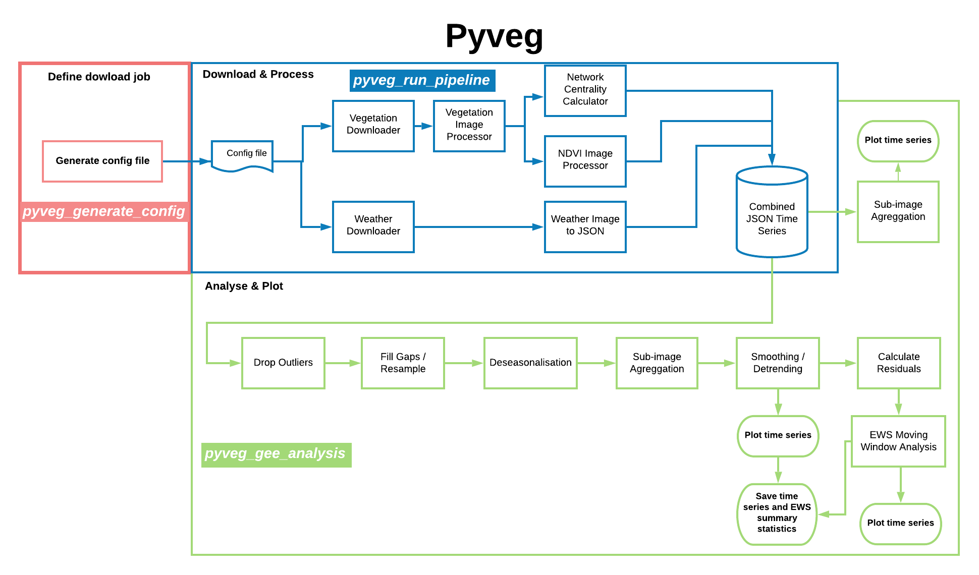 The
Thepyveg program flow.
The full ReadTheDocs documentation for this pyveg can be found in this link.
This page contains an installation guide, and some usage examples for this package.
Installation
pyveg requires Python 3.6 or greater. To install, start by creating a fresh conda environment.
conda create -n veg python=3.7
conda activate veg
Get the source.
git clone https://github.com/alan-turing-institute/monitoring-ecosystem-resilience.git
Enter the repository and check out a relevant branch if necessary (the develop branch contains the most up to date stable version of the code).
cd monitoring-ecosystem-resilience
git checkout develop
Install the package using pip.
pip install .
If you are using Windows and encounter issues during this stage, a solution may be found here: https://github.com/NREL/OpenOA/issues/37. If you plan on making changes to the source code, you can instead run pip install -e ..
Before using the Google Earth Engine API, you need to sign up with a Google account here, and authenticate. To authenticate, run
earthengine authenticate
A new browser window will open. Copy the token from this window to the terminal prompt to complete the authentication process.
Google Earth Engine
Google Earth Engine (GEE) is a powerful tool for obtaining and analysing satellite imagery. This directory contains some useful scripts for interacting with the Earth Engine API. The earth engine API is installed automatically as part of the pyveg package installation. If you wish to install it separately, you can follow the instructions here.
Downloading data from GEE with pyveg
Downloading data from GEE using the CLI
To run a pyveg download job, use
pyveg_run_pipeline --config_file <path to config>
The download job is fully specified by a configuration file, which you point to using the --config_file argument. A sample config file is found at pyveg/configs/config_all.py. You can also optionally specify a string to identify the download job using the --name argument.
Note that we use the GEE convention for coordinates, i.e. (longitude,latitude).
Generating a download configuration file
To create a configuration file for use in the pyveg pipeline described above, use the command
pyveg_generate_config
this allows the user to specify various characteristics of the data they want to download via prompts. The list in order is as follows:
--configs_dir: The path to the directory containing the config file, with a default optionpyveg/configs.--collection_name: The name of the dataset used in the collection, either Sentinel2, or Landsat 8, 7, 5 or 4.--latitude: The latitude (in degrees north) of the centre point of the image collection.--longitude: The longitude (in degrees east) of the centre point of the image collection.--country: The country (for the file name) can either be entered, or use the specified coordinates to look up the country name from the OpenCage database.--start_date: The start date in the format ‘YYYY-MM-DD’, the default is ‘2015-01-01’ (or ‘2019-01-01’ for a test config file).--end_date: The end date in the format ‘YYYY-MM-DD’, the default is today’s date (or ‘2019-03-01’ for a test config file).--time_per_point: The option to run the image collection either monthly (‘1m’) or weekly (‘1w’), with the default being monthly.--run_mode: The option to run time-consuming functions on Azure (‘batch’) or running locally on your own computer (‘local’). The default is local. For info about running on Azure go here.--output_dir: The option to write the output to a specified directory, with the default being the current directory.--test_mode: The option to make a test config file, containing fewer months and a subset of sub-images, with a default option to have a normal config file.By choosing the test config file, the start and end dates (see below) are defaulted to cover a smaller time span.
It is recommended that the test config option should be used purely to determine if the options specified by the user are correct.
--n_threads: Finally, how many threads the user would like to use for the time-consuming processes, either 4 (default) or 8.
For example:
pyveg_generate_config --configs_dir "pyveg/configs" --collection_name "Sentinel2" --latitude 11.58 --longitude 27.94 --start_date "2016-01-01" --end_date "2020-06-30" --time_per_point "1m" --run_mode "local" --n_threads 4
This generates a file named config_Sentinel2_11.58N_27.94E_Sudan_2016-01-01_2020-06-30_1m_local.py along with instructions on how to use this configuration file to download data through the pipeline, in this case the following:
pyveg_run_pipeline --config_file pyveg/configs/config_Sentinel2_11.58N_27.94E_Sudan_2016-01-01_2020-06-30_1m_local.py
Individual options can be specified by the user via prompt. The options for this can be found by typing pyveg_generate_config --help.
More Details on Downloading
During the download job, pyveg will break up your specified date range into a time series, and download data at each point in the series. Note that by default the vegetation images downloaded from GEE will be split up into 50x50 pixel images, vegetation metrics are then calculated on the sub-image level. Both colour (RGB) and Normalised Difference Vegetation Index (NDVI) images are downloaded and stored. Vegetation metrics include the mean NDVI pixel intensity across sub-images, and also network centrality metrics, discussed in more detail below.
For weather collections e.g. the ERA5, due to coarser resolution, the precipitation and temperature “images” are averaged into a single value at each point in the time series.
Rerunning partially succeeded jobs
The output location of a download job is datestamped with the time that the job was launched. The configuration file used will also be copied and datestamped, to aid reproducibility. For example if you run the job
pyveg_run_pipeline --config_file pyveg/configs/my_config.py
there will be a copy of my_config.py saved as pyveg/configs/cached_configs/my_config_<datestamp>.py. This also means that if a job crashes or timeouts partway through, it is possible to rerun, writing to the same output location and skipping parts that are already done by using this cached config file. However, in order to avoid a second datestamp being appended to the output location, use the --from_cache argument. So for the above example, the command to rerun the job filling in any failed/incomplete parts would be:
pyveg_run_pipeline --config_file pyveg/configs/cached_configs/my_config_<datestamp>.py --from_cache
Using Azure for downloading/processing data
If you have access to Microsoft Azure cloud computing facilities, downloading and processing data can be sped up enormously by using batch computing to run many subjobs in parallel. See here for more details.
Downloading data using the API
Although pyveg has been mostly designed to be used with the CLI as shown above, we can also use pyveg functions through the API. A tutorial of how to download data this way is included in the notebooks/tutorial_download_and_process_gee_images.ipynb notebook tutorial.
Analysing the Downloaded Data with pyveg
Analysing the Downloaded Data using the CLI
Once you have downloaded the data from GEE, the pyveg_gee_analysis command allows you to process and analyse the output. To run:
pyveg_gee_analysis --input_dir <path_to_pyveg_download_output_dir>
The analysis code preprocesses the data and produces a number of plots. These will be saved in an analysis/ subdirectory inside the <path_to_pyveg_download_output_dir> directory.
Note that in order to have a meaningful analysis, the dowloaded time series should have at least 4 points (and more thant 12 for an early warning analysis) and not being the result of a “test” config file, in this case the analysis fails.
The commands also allows for other options to be added to the execution of the script (e.g. run analysis from a downloaded data in Azure blob storage, define a different output directly, don’t include a time series analysis, etc), which can be displayed by typing:
pyveg_gee_analysis --help
The analysis script executed with the pyveg_gee_analysis command runs the following steps:
Preprocessing
pyevg supports the following pre-processing operations:
Identify and remove outliers from the time series.
Fill missing values in the time series (based on a seasonal average), or resample the time series using linear interpolation between points.
Smoothing of the time series using a LOESS smoother.
Calculation of residuals between the raw and smoothed time series.
De-seasonalising (using first differencing), and detrending using STL.
Plots
In the analysis/ subdirectory, pyveg creates the following plots:
Time series plots containing vegetation and precipitation time series (seasonal and de-seasonalised). Plots are labelled with the AR1 of the vegetation time series, and the maximum correlation between the Vegetation and precipitation time series.
Auto-correlation plots for vegetation and precipitation time series (seasonal and de-seasonalised).
Vegetation and precipitation cross-correlation scatterplot matrices.
STL decomposition plots.
Resilience analysis:
ewstoolsresilience plots showing AR1, standard deviation, skewness, and kurtosis using a moving window.Smoothing filter size and moving window size Kendall tau sensitivity plots.
Significance test.
Running the analysis using the API
Although pyveg has been mostly designed to be used with the CLI as shown above, we can also use pyveg functions through the API. A tutorial of how to run the data analysis in this way is included in the notebooks/tutorial_analyse_gee_data.ipynb notebook tutorial.
Other functionalities of pyveg
Analysis summary statistics data
The analyse_pyveg_summary_data.py functionality processes collections of data produced by the main pyveg pipeline described in the section above (download + time series analysis for different locations and time periods) and creates a number of plots of the summary statistics of these time series.
To run this analysis in Python, there is an entrypoint defined. Type:
pyveg_analysis_summary_data --input_location <path_to_directory_with_collection_summary_statistics>
if you wish you can also specify the outpur_dir where plots will be saved. Type:
pyveg_analysis_summary_data --help
to see the extra options.
Pattern simulation
The generate_patterns.py functionality originates from some Matlab code by Stefan Dekker, Willem Bouten, Maarten Boerlijst and Max Rietkerk (included in the “matlab” directory), implementing the scheme described in:
Rietkerk et al. 2002. Self-organization of vegetation in arid ecosystems. The American Naturalist 160(4): 524-530.
To run this simulation in Python, there is an entrypoint defined. Type:
pyveg_gen_pattern --help
to see the options. The most useful option is the --rainfall parameter which sets a parameter (the rainfall in mm) of the simulation - values between 1.2 and 1.5 seem to give rise to a good range of patterns. Other optional parameters for generate_patterns.py allow the generated image to be output as a csv file or a png image. The --transpose option rotates the image 90 degrees (this was useful for comparing the Python and Matlab network-modelling code). Other parameters for running the simulation are in the file patter_gen_config.py, you are free to change them.
Network centrality
There is an entrypoint defined in setup.py that runs the main function of calc_euler_characteristic.py:
pyveg_calc_EC --help
will show the options.
--input_txtallows you to give the input image as a csv, with one row per row of pixels. Inputs are expected to be “binary”, only containing two possible pixel values (typically 0 for black and 255 for white).--input_imgallows you to pass an input image (png or tif work OK). Note again that input images are expected to be “binary”, i.e. only have two colours.--sig_threshold(default value 255) is the value above (or below) which a pixel is counted as signal (or background)--upper_thresholddetermines whether the threshold above is an upper or lower threshold (default is to have a lower threshold - pixels are counted as “signal” if their value is greater-than-or-equal-to the threshold value).--use_diagonal_neighbourswhen calculating the adjacency matrix, the default is to use “4-neighbours” (i.e. pixels immediately above, below, left, or right). Setting this option will lead to “8-neighbours” (i.e. the four neighbours plus those diagonally adjacent) to be included.--num_quantilesdetermines how many elements the output feature vector will have.--do_ECCalculate the Euler Characteristic to fill the feature vector. Currently this is required, as the alternative approach (looking at the number of connected components) is not fully debugged.
Note that if you use the -i flag when running python, you will end up in an interactive python session, and have access to the feature_vec, sel_pixels and sc_images variables.
Examples:
pyveg_calc_EC --input_txt ../binary_image.txt --do_EC
>>> sc_images[50].show() # plot the image with the top 50% of pixels (ordered by subgraph centrality) highlighted.
>>> plt.plot(list(sel_pixels.keys()), feature_vec, "bo") # plot the feature vector vs pixel rank
>>> plt.show()
Contributing
We welcome contributions from anyone who is interested in the project. There are lots of ways to contribute, not just writing code. See our Contributor Guidelines to learn more about how you can contribute and how we work together as a community.
Licence
This project is licensed under the terms of the MIT software license.